Function Approximation: Interpolation, RBFs and Optimised Nodes
Often you only know a function at a handful of points, but need its value everywhere in between. Getting this right is at the heart of simulations and data analysis. I compared several classic ways of filling in the gaps, found out where each one breaks down, and used optimisation to choose better points.
- Individual project.
- Sep 2026
- Completed
- Python · NumPy · autograd · matplotlib · Interpolation · Optimisation
Problem
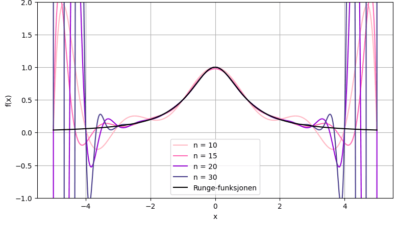
Given a function's values at points, how do you best approximate it everywhere else? The obvious answer, fitting one polynomial through equally spaced points, can fail badly: for Runge's function the error grows near the ends as you add more points.
The project compared global polynomial interpolation, piecewise interpolation and radial basis functions (RBFs). It asked for predictions before experiments, and explanations whenever theory and numerics disagreed.
Technical skills
- Polynomial interpolation (Lagrange) with equidistant and Chebyshev nodes
- Error analysis: interpolation error bounds, max-norm and 2-norm estimates, convergence rates
- Piecewise polynomial interpolation and run-time measurements
- Radial basis function interpolation and condition numbers of linear systems
- Gradient descent with backtracking line search
- Automatic differentiation with autograd
- Scientific Python: NumPy, matplotlib and Jupyter
Approach
Lagrange interpolation
Equidistant vs Chebyshev nodes, with error measured in the max-norm and 2-norm and compared with theoretical error bounds.
Piecewise interpolation
Low-degree polynomials on many subintervals; convergence rates and measured run times compared with global interpolation.
Radial basis functions
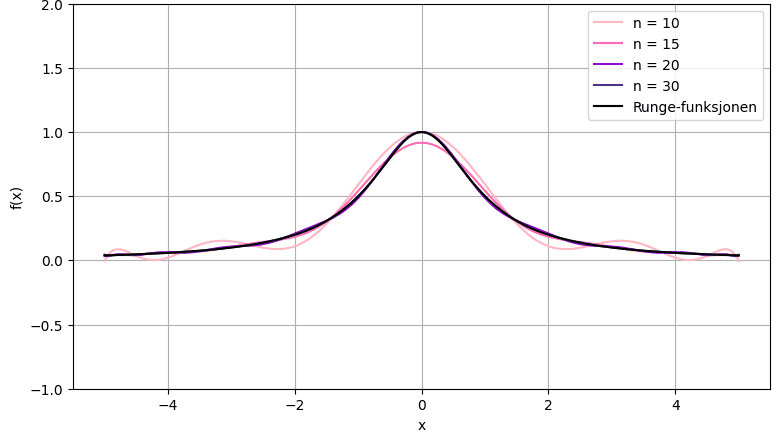
Gaussian RBF interpolation, and how the shape parameter trades accuracy against the conditioning of the linear system.
Optimising the nodes
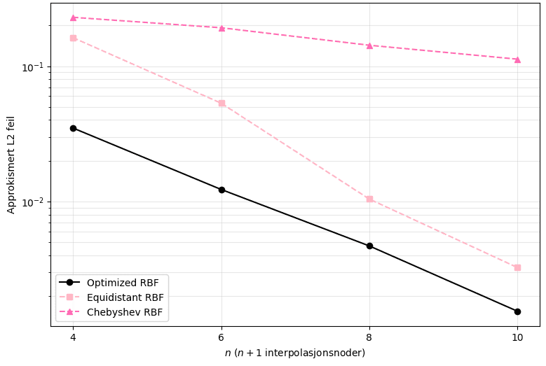
Gradient descent with backtracking, using automatic differentiation (autograd) to optimise node positions and together.
Results
The full notebook with code, plots and discussion is on GitHub.