Numerical Boundary-Value Problems and the Josephson Effect
Superconductors can carry current with zero resistance, even across a thin layer of ordinary metal. This effect is used in quantum computers and extremely sensitive sensors. We first wrote and tested our own tools for solving the equations involved, then used numerical methods to compute that current.
- Group of 3, with Andrine Holen and Emily Ann Mercer. We each worked through every task, compared approaches and results, and then split the final write-up.
- Apr 2026
- Completed
- A
- Python · NumPy · SciPy · matplotlib
Problem
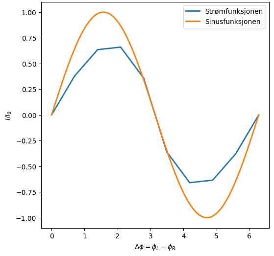
When two superconductors are separated by a thin normal metal, a current can flow between them with zero resistance, driven only by the difference in their quantum phases. This Josephson effect is the key component of superconducting qubits and ultra-sensitive magnetic sensors.
Describing it requires solving a nonlinear boundary-value problem: the solution is fixed at both ends, not just at the start. The project had two parts: build reliable solvers ourselves, then apply numerical methods to the junction.
Technical skills
- Adaptive Runge–Kutta methods with error estimation and step-size control
- Root finding (secant method) and the shooting method for boundary-value problems
- Solving nonlinear boundary-value problems with
scipy.integrate.solve_bvp - Complex linear algebra: rewriting complex matrix equations as real vector systems
- Continuation methods: reusing solutions as initial guesses
- Numerical integration (Simpson's rule) and verification against exact solutions
Approach
Adaptive Runge–Kutta solver
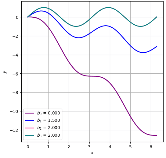
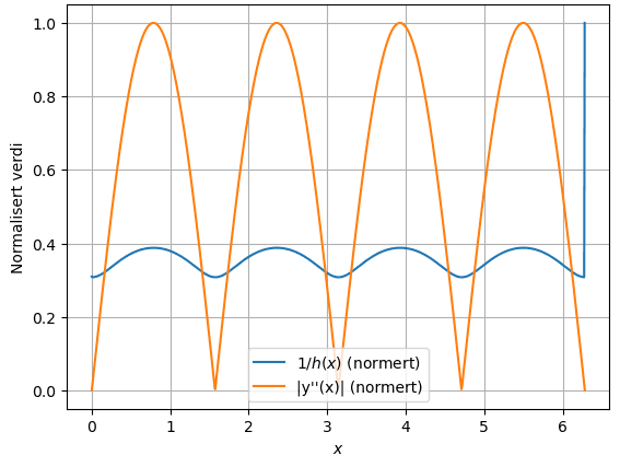
Takes small steps where the solution changes quickly and large steps where it does not.
Shooting method
Guess the missing initial slope, integrate, and correct the guess with a root finder until the far boundary is hit.
Verify
Compare with exact solutions and SciPy's boundary-value solver.
The physics
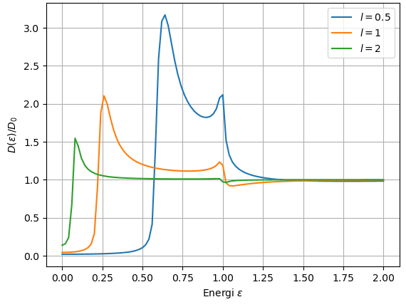
Solve the Usadel equations for the junction with SciPy, then compute the density of states and the supercurrent.
Results
The full notebook with all calculations and plots is on GitHub.